Data | Data Science and AI
Combining Neo4J and Hadoop (part II) 
Kris Geusebroek 17 Jan, 2013


A single, reliable source of truth is what every business and decision-maker hopes for. This is also what we pursue as Data professionals. How can we ensure that two different dashboards, or any other data consumer, is calculating the metrics (revenue, for example) in the same way? Moving metric definitions out of the BI and consumption layer and into the modeling layer allows data teams and stakeholders to feel confident that different business units are working from the same metric definitions, regardless of their tool of choice. If a metric definition changes, it’s refreshed everywhere it’s invoked and creates consistency across all applications.
This is where a Semantic Layer plays an important role. It is a virtual layer that sits between the raw data and the end-user, providing a simplified and unified view of the data. It acts as a translation layer, transforming complex data sources into a more understandable and business-friendly format. The Semantic Layer abstracts away the complexities of the underlying data structures, allowing users to interact with the data using familiar business terms and concepts.
In summary, the Semantic Layer plays a crucial role in enhancing data accessibility, consistency, and usability, making it an essential component in modern data management and analytics architectures.
In the most recent release (as of Sep/23 – v1.6), dbt has re-launched the Semantic Layer, now powered by MetricFlow (you can find more about MetricFlow here).
This update simplifies the process of defining and using critical business metrics by centralizing metrics definitions. When a metric definition changes in dbt, it is automatically updated everywhere it is used, ensuring consistency across all applications.
The concept of OBT (One Big Table) has been widely adopted by dbt developers, denormalizing the data in each of the layers, from staging, to intermediate and marts. However, as projects grow, multiple big tables start to emerge, resulting in duplicated metrics in different places and increasing the complexity and maintenance efforts.
The new dbt Semantic Layer introduces a paradigm shift by using normalized data instead of denormalized. Semantic Models, Dimensions, and Metrics are defined, while MetricFlow handles the rest, ensuring a more efficient and streamlined approach. For a Semantic Layer implementation, it is usual – and commonly recommended – to use directly a staging model instead of a mart to build the Semantic Model and Metrics.
This guide was made based on this official post from dbt.
Let’s use this repository as reference for our Semantic Layer implementation. There, we have a simple dbt project, which applies basic transformations in a NYC Taxi trips public database. The project is set using the recommended layers – source → staging → intermediate → marts. For this example, we will keep things simple and create our Semantic Models and Metrics using a mart.
All Semantic Layer definitions (semantic_models and metrics), are placed in the .yml files. This will increase exponentially the number of lines, so instead of having a single .yml for each folder, we will create one file for each model.
To begin our implementation, let’s checkout to the start-here branch.
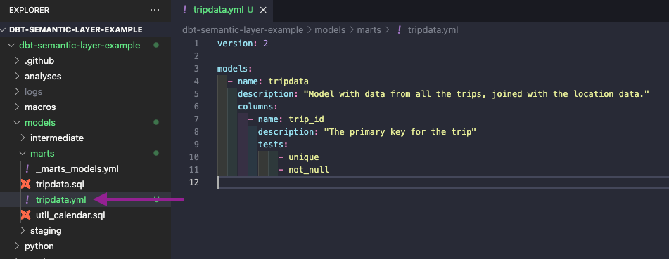
First, we will create a new file named tripdata.yml, and move our current configurations of the tripdata model there.
Next, we will start to build our Semantic Model definitions.
There are two main pieces for our Semantic Layer settings: semantic_models and metrics.
We will begin by defining the semantic_models.
semantic_models:
  - name: tripdata
    defaults:
      agg_time_dimension: pickup_date
    description: |
      Tripdata fact table. This table is at the trip grain with one row per trip.
    #The name of the dbt model and schema
    model: ref('tripdata')
Nested into semantic_models, we will define entities, measures and dimensions.
For the entities, these correspond to the keys of a table. The entities are also used to join different tables. Usually, the ids columns are defined as entities.
  entities:
      - name: trip_id
        type: primary
      - name: vendor
        type: foreign
        expr: vendor_id
      - name: pickup_location
        type: foreign
        expr: pickup_location_id
      - name: dropoff_location
        type: foreign
        expr: dropoff_location_id
Next, we will define the measures. Here is where we define how our data will be aggregated. We can define, for example, sum for numeric columns, count and count_distinct.
You can think of measures as the aggregation functions in SQL (SUM, COUNT, etc)
  measures:
      - name: total_amount
        description: The total value for each trip.
        agg: sum
      - name: trip_count
        expr: 1
        agg: sum
      - name: tip_amount
        description: The total tip paid on each trip.
        agg: sum
      - name: passenger_count
        description: The total number of passengers on each trip.
        agg: sum
For the dimensions, they define the granularity of our metrics. For example, the following parameters would allow us to calculate the total_amount for each pickup_borough, or pickup_date.
You can think of dimensions as the columns that are present in a group by in SQL.
  dimensions:
      - name: pickup_date
        type: time
        type_params:
          time_granularity: day
      - name: pickup_borough
        type: categorical
      - name: dropoff_borough
        type: categorical
      - name: traject_borough
        type: categorical
Finally, we will set the metrics. They are what will be exposed for the consumers, built on top of measures and other metrics.
There are multiple options and settings available for metrics (filters, types, type_params, etc), you can check all of them here.
For this example, let’s create just a simple one.
metrics:
  - name: total_amount
    description: Sum of total trip amount.
    type: simple
    label: Total Amount
    type_params:
      measure: total_amount
Our final tripdata.yml file should be the following.
version: 2

models:
  - name: tripdata
    description: "Model with data from all the trips, joined with the location data."
    columns:
      - name: trip_id
        description: "The primary key for the trip"
        tests:
            - unique
            - not_null

semantic_models:
  - name: tripdata
    defaults:
      agg_time_dimension: pickup_date
    description: |
      Tripdata fact table. This table is at the trip grain with one row per trip.
    #The name of the dbt model and schema
    model: ref('tripdata')

    entities:
      - name: trip_id
        type: primary
      - name: vendor
        type: foreign
        expr: vendor_id
      - name: pickup_location
        type: foreign
        expr: pickup_location_id
      - name: dropoff_location
        type: foreign
        expr: dropoff_location_id

    measures:
      - name: total_amount
        description: The total value for each trip.
        agg: sum
      - name: trip_count
        expr: 1
        agg: sum
      - name: tip_amount
        description: The total tip paid on each trip.
        agg: sum
      - name: passenger_count
        description: The total number of passengers on each trip.
        agg: sum

    dimensions:
      - name: pickup_date
        type: time
        type_params:
          time_granularity: day
      - name: pickup_borough
        type: categorical
      - name: dropoff_borough
        type: categorical
      - name: traject_borough
        type: categorical

metrics:
  - name: total_amount
    description: Sum of total trip amount.
    type: simple
    label: Total Amount
    type_params:
      measure: total_amount
You can see the code we have so far in the branch create-semantic-layer.
That’s it, our first Semantic Layer metric is ready!
There is only one thing missing for it to work: MetricFlow requires a metricflow_time_spine.sql model for the Semantic Layer to work properly. Therefore, we will create it in the marts folder.
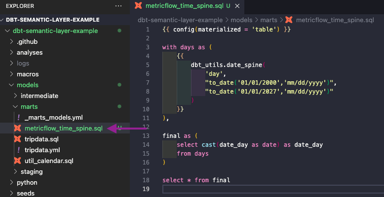
You can use the following code in the new model. It requires the dbt_utils package, which you can add in your packages.yml file (instructions here).
{{ config(materialized = 'table') }}

with days as (
    {{
        dbt_utils.date_spine(
            'day',
            "to_date('01/01/2000','mm/dd/yyyy')",
            "to_date('01/01/2027','mm/dd/yyyy')"
        )
    }}
),

final as (
    select cast(date_day as date) as date_day
    from days
)

select * from final
You can see the code we have so far in the branch create-time-spine.
Now, all that is left is to commit and push our changes.
Currently, it is only supported to connect to the Semantic Layer using dbt Cloud, so this is the path we will take in the next section.
Before we start, there are a few conditions we have to meet to be able to configure the Semantic Layer in dbt Cloud, you can read them here.
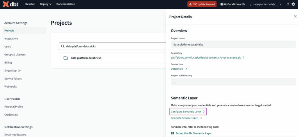
First, we will configure the credentials the Semantic Layer will use to connect to the Data Warehouse. To do so, we have to navigate to Account Settings → Projects → [Select your project] → Configure Semantic Layer.
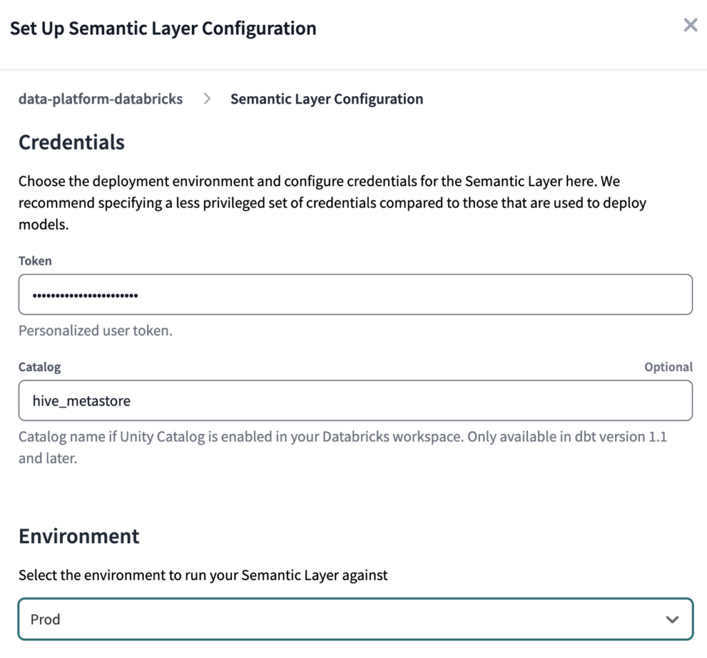
Depending on which warehouse you are using, the fields that you have to fill may be different. In our case, we used Databricks, therefore we have to set a Token and catalog (if using Unity Catalog).
For the Environment, select the production one – Prod in our case.
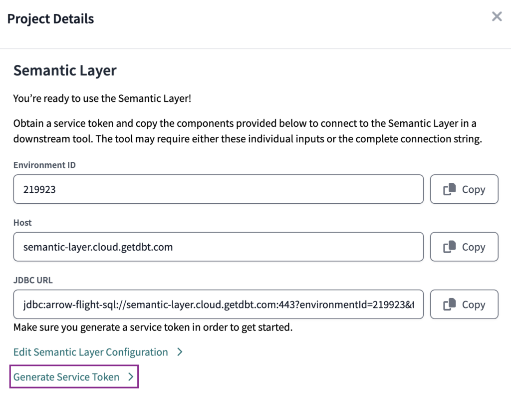
Once the credentials are correctly set, the Semantic Layer details will be visible. We will save the Environment ID value for later use.
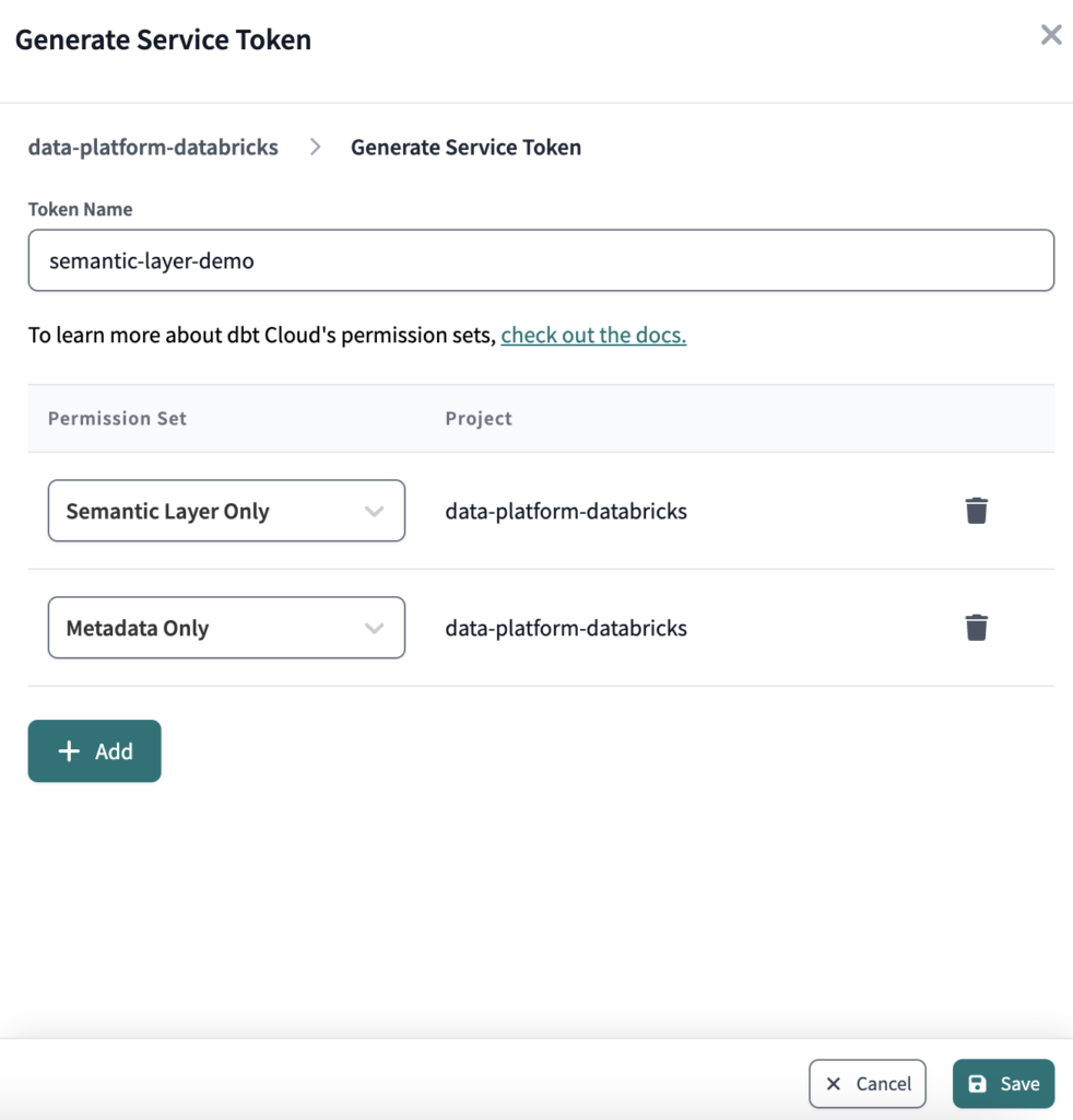
Finally, we will generate a service token that will be used to access dbt Cloud’s Semantic Layer API.
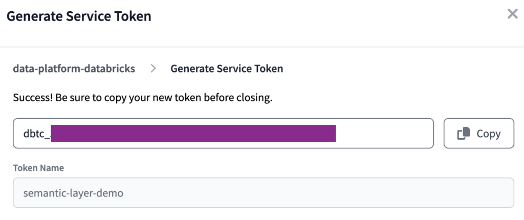
Copy the value of the token before closing the window – it will be shown only once and we will need it later on.
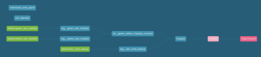
That’s it from the dbt Cloud side! If you want, you can also navigate to the Develop IDE and check your lineage.
The new Metric should be there and look something like this.
Now that we have our first metric defined, how can we actually see the result? Since there are still only a few integrations available, it is not that easy to check the results. Since the goal of this first implementation is to try and get familiar with the new dbt Semantic Layer, we will use DBeaver to connect with it – of course this isn’t a production-ready setup, but it is still a public-beta of the dbt Semantic Layer, after all.
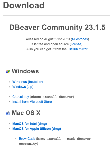
The first step is to download and install DBeaver on your computer. You can find it here.
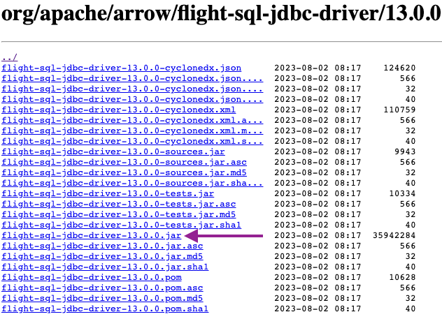
For this setup, we will connect to dbt Semantic Layer using ArrowFlightSQL. Therefore, the next step will be to download the latest version of ArrowFlightSQL Driver. You can find it here – Download version 12 or later.
Note that if you search for the Driver at Google, you may find Dremio’s website, which leads you to an older version.
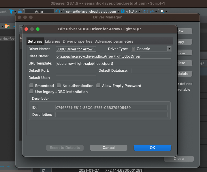
Next, we will open the Driver Manager, under the Database tab, and create a New driver. We will set the values as follows.
Driver Name: JDBC Driver for Arrow Flight SQL
Driver Type: Generic
Class Name: org.apache.arrow.driver.jdbc.ArrowFlightJdbcDriver
URL Template: jdbc:arrow-flight-sql://{host}:{port}
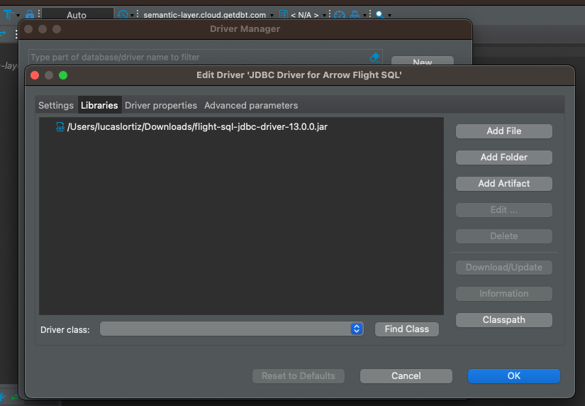
Under the Libraries tab, we will click on Add File and select the driver we downloaded in the previous step.
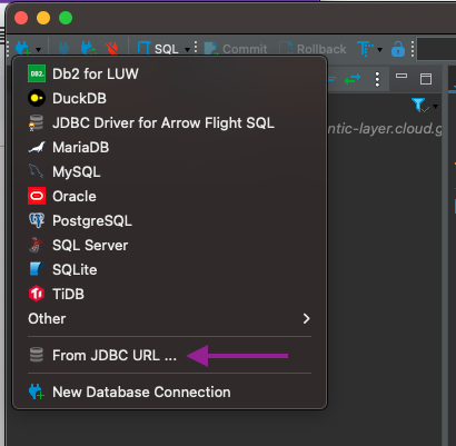
Now, it is time to create our connection. We will first click to add a new connection and select From JDBC Url…
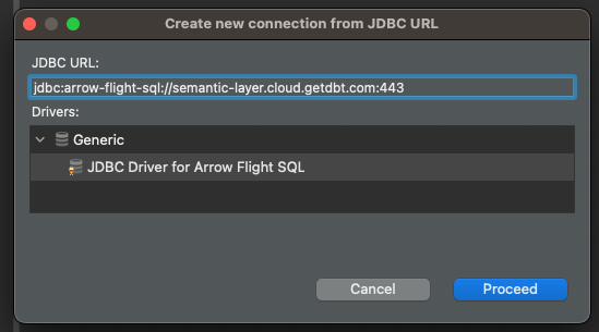
We will set the URL as jdbc:arrow-flight-sql://semantic-layer.cloud.getdbt.com:443
Once we insert this value, it will automatically load our recently-created Driver. Just click on Proceed.
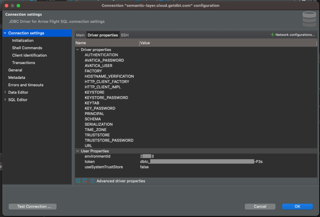
Now, we will set the settings specific to this connection. The main thing here is to add the correct connection parameters. To do so, navigate to the Driver properties tab, right-click the User Properties item and select Add new property. We will create three properties: environmentId, token and useSystemTrustStore. The first two we have gathered in the previous section, for the last, we will set as false.
Once everything is set, click on Test Connection… and confirm in the windows that will open.
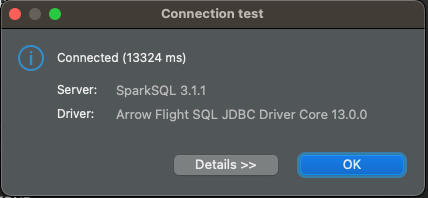
That’s it! Our connection with dbt Semantic Layer is set, now all that is left to do is to query our metrics.
Here you can find all the specifics about querying your dbt Semantic Layer, below you can find two examples.
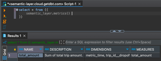
To retrieve all the metrics created.
select * from {{
    semantic_layer.metrics()
}}
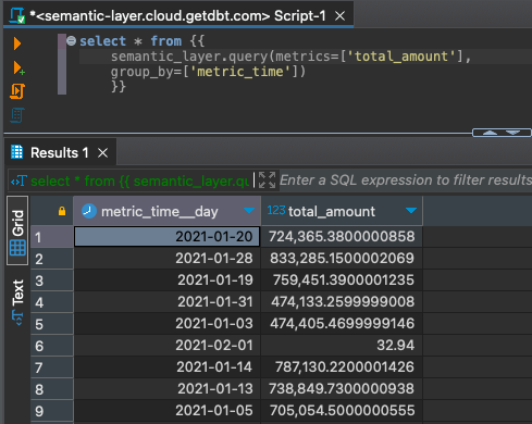
To retrieve the values of a metric, grouped by each time grain.
select * from {{
    semantic_layer.query(metrics=['total_amount'],
    group_by=['metric_time'])
    }}
Implementing a Semantic Layer provides numerous benefits for data management in projects of all sizes. By centralizing metric definitions and normalizing data, a Semantic Layer simplifies the process of defining and using critical business metrics while ensuring consistency across applications.
In that sense, dbt Semantic Layer can become a valuable ally in ensuring the correct source of truth. It is a new feature, with many developments, best practices to be defined, and improvements to be made, but the sooner you get familiar with the tool and concepts, the better you will be able to implement it in a production-grade way as the market evolves.